This paper presents an efficient history matching approach that simultaneously integrates 4D repeat seismic surveys with well production data. This approach is particularly well-suited for the calibration of the reservoir properties of high-resolution geologic models because the seismic data are areally dense but sparse in time, while the production data are continuous in time but averaged over interwell spacing. The joint history matching is performed using streamline-based sensitivities derived from either finite-difference or streamline-based flow simulation.
Introduction
Previous studies have made attempts at quantitative 4D seismic history matching. However, the reconciliation of reservoir model heterogeneity with temporal changes in seismic attributes remains a particularly complex task. Several dynamic data integration algorithms have been proposed in the literature, which can be categorized broadly into three data integration levels: (1) reservoir-simulation-based integration between the pressure and saturation estimates inverted from seismic observation data and the direct simulated saturation and pressure responses, (2) petroelastic-based integration between the seismic inverted rock elastic properties derived from a geophysical inversion and the simulated rock elastic responses from the simulated saturation and pressure responses by means of petroelastic models, and (3) seismic-forward-model-based integration between the direct seismic traces attributes and the simulated seismic responses by means of seismic wave propagation modeling.
The seismic-forward-model-based seismic data integration approach uses direct seismic trace data and circumvents the uncertainties associated with the seismic-inversion process. The general workflow for generating synthetic seismic data from a reservoir simulation model generally involves (1) static reservoir properties on the simulation grid, (2) simulation of dynamic pressure and fluid saturations at each cell, (3) computation of seismic elastic properties, and (4) simulation of the seismic attribute by applying a seismic wave propagation model over the reservoir interval and the overburden rock.
This study examines both reservoir-simulation-based calibration and rock-physics-based calibration. In the first instance, the authors calibrate against time-lapse changes in both pressure and saturation. In the second instance, they calibrate against the time-lapse change in acoustic impedance. In both cases, the inversion will provide local updates to the reservoir model using analytic streamline-based sensitivity calculations.
Background and Methodology
The approach used here relies on the use of streamlines to relate the reservoir properties to the dynamic reservoir response: production, pressure, and time-lapse seismic response. Establishing these relations, also called sensitivities, is crucial to the data-integration process. Streamlines are used extensively to describe the flow field and to calculate the fluid tracer time of flight along each streamline. The time of flight acts as a spatial coordinate along the lines. However, the proposed approach does not rely on the use of a streamline simulator and is well-suited for both conventional finite-difference reservoir simulators and streamline simulators. For streamline simulators, the streamline trajectories and time of flight are readily available. However, for finite-difference simulation, the streamline and time of flight are obtained by post-processing of the finite-difference velocity field. For the mathematical details of sensitivities calculations, please see the complete paper.
History-Matching Applications
Five-Spot Synthetic Case. A synthetic 2D model illustrates the proposed inversion approach. The model contains 50×50×1 cells with a five-spot well configuration: one injector in the center and four producers at the corners. Wells are constrained by the historical (constant) reservoir flow rates.
The approach involves first matching of the time-lapse pressure changes followed by matching of the saturation changes. Finally, well-by-well water-cut matching is performed using the generalized travel time inversion method. The reasoning behind the sequential approach is that the pressure data is well-suited to capture large-scale (global) variation while saturation and production data capture small-scale (local) variation.
Pressure-change data-integration results show significant reduction in the objective function within a few iterations. The updated permeability field appears to identify the low-permeability barrier. Also, the time-lapse pressure change response improved significantly compared with the initial model. Next, saturation changes are integrated into the updated model from the previous step. Finally, the generalized travel time inversion is applied to match the well-by-well water-cut data. The final model responses are well matched to the reference model both for bottomhole pressure and water-cut data with corresponding improvements of time-lapse pressure and saturation change responses. These results confirm that the consistent integration of both time-lapse pressure and saturation changes together with production data can constrain the history-matching solution effectively with the proposed approach.
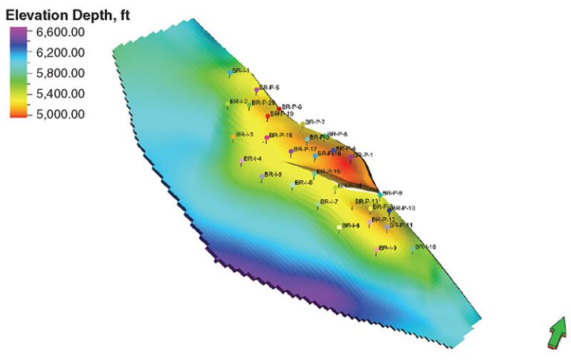
The Brugge Field Case. The Brugge field case was designed for a Society of Petroleum Engineers benchmark project to test the combined use of history matching and waterflooding optimization methods in a closed-loop workflow. The structure of the Brugge field consists of an east/west elongated half-dome with a large boundary fault at its northern edge and one internal fault with a modest throw, as shown in Fig. 1. The dimensions of the field are roughly 10×3 km. The reservoir model contains more than 40,000 active grid cells, 20 producers located in the center of the dome, and 10 infill water injectors located in the surrounding aquifer to provide additional pressure support. A total of 104 realizations were generated by four classes of control parameters: (1) facies association, (2) facies modeling, (3) porosity, and (4) permeability. Production data are given in the form of water and oil rates and bottomhole pressure at each of the 20 producers for the 10 years of production. Inverted 4D seismic data in terms of pressure and saturation changes between the time lapse of 10 years are also provided. Pressure and saturation changes were calculated as vertically averaged values over the four reservoir zones in nine layers, representative for the seismic resolution with added noise. These data sets were used as observation data to calibrate reservoir permeability to minimize the differences of the observed and simulated time-lapse pressure and saturation changes as well as the production data. One of the challenging aspects of this application is the long gap of the time-lapse data. During the 10 years of production, the reservoir drive mechanism has evolved from primary depletion to secondary recovery with the down-dip water injection. Accordingly, the dynamic changes of the reservoir pressure and saturation must be accounted for to integrate the available time-lapse data.
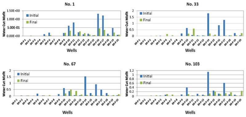
First, pressure-change data is used to calibrate the models. Next, water saturation change is integrated to update the models. Finally, the generalized travel-time inversion is applied to integrate water-cut data into the models. The improvements in well-by-well production response match are shown in Fig. 2. Overall, the magnitude of pressure changes reduced from initial model responses for all realizations. As for water-saturation changes, the improvements of the magnitude of changes and the distribution of water fronts are more evident in the final updated models.
The Norne Field Case. The Norne field was discovered in December 1991, and development drilling began in August 1996. Oil production started in November 1997. The field has high-quality 4D seismic data, production data, and well logs in addition to the reservoir model.
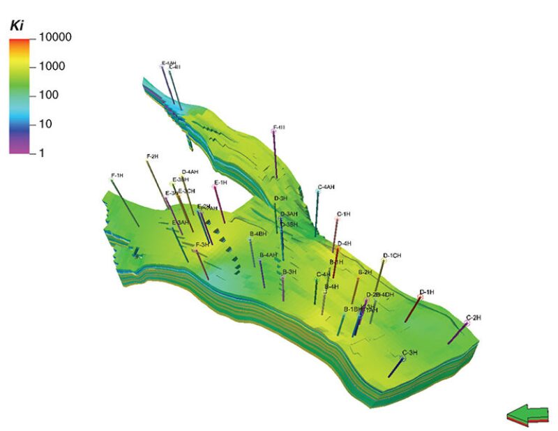
The practical feasibility of the approach was demonstrated by carrying out full-field history matching of the Norne field. The reservoir model consists of 44,431 active cells and contains 36 wells (nine injectors and 27 producers), as shown in Fig. 3. The time frame from 1997 to 2006 was considered as the history-matching period. The actual simulation model containing all information and properties was provided by the operator. In addition, production and injection data from 1997 to the end of 2006 and multiple sets of 4D seismic data for the same period were provided. The production data include water, oil, and gas rates and bottomhole pressures at the producers. The seismic data were externally processed and provided for the model calibration as near, mid, far, and full offset stacked 3D volumes of the reflection amplitude together with the corresponding horizons for the top and base of the reservoir. Also, the time-lapse differences of the reflection amplitude were provided with interpreted horizons used for identification of movement of the water/oil contacts.
Petroelastic Model. Unlike the Brugge field case, in which interpreted saturation and pressure changes are provided as part of the field data, this is a much more realistic case, in which seismic response is provided instead. Consequently, a petroelastic model must be added to the strategy of using streamline-based sensitivities for the inversion problem and sensitivities to changes in reservoir properties must be developed.
A petroelastic model is a set of equations that relates reservoir properties (pore volume, pore fluid saturations, reservoir pressures, and rock composition) to seismic rock elastic parameters. Variations in rock elastic properties are functions of temperature, compaction, fluid saturation, and reservoir pressure, although the effects of temperature may be neglected in this field. Please see the complete paper for the equations.
Seismic Data Processing. The first step in the data-calibration procedure is to invert the seismic volumes of reflection amplitude to changes in acoustic impedance. Using commercial software, the authors conducted seismic data processing that consisted of (1) time to depth data conversion, (2) well log quality check and acoustic impedance log calculation, and (3) genetic inversion for generating an acoustic impedance map from the seismic amplitude data.
Global to Local Hierarchical History-Matching Workflow. The reservoir model provided by the operator was already calibrated to match the reservoir energy (regional pressure and pore volume). The authors adjusted fault transmissibility multipliers, regional relative permeability parameters, and large-scale absolute permeability and porosity heterogeneity using regional and constant multipliers. The objective was to update the permeability minimally at locations and scales required to improve large-scale transport within the reservoir induced by the production, water injection, and aquifer support and to leave the prior otherwise unchanged. A hierarchical history-matching workflow that consisted of two stages, a global update and a local update, was applied.
Local Step Time-Lapse Acoustic Impedance Change Data and Production Data Integration. After the global calibration step, a few candidate models were selected for the local updates by a cluster analysis in the objective space. For the local update, the sensitivity of the acoustic impedance with respect to gridblock permeability was needed.
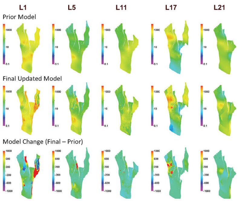
The history matching follows a sequential approach. To start with, the pressure effects on acoustic impedance changes are integrated to calibrate the model. Next, the saturation effects on the acoustic impedance changes are integrated to update the model. Water saturation sensitivity and gas saturation sensitivity are separately integrated in the inversion process. The majority of the reduction of the acoustic impedance change data misfit was achieved in the global step of the model calibration. Finally, the generalized travel-time inversion is applied to integrate water-cut data. The final model responses in terms of acoustic-impedance changes are compared in Fig. 4. Overall, the misfit of the time-lapse acoustic-impedance change and well-production response are improved substantially from the prior model.
This article, written by Special Publications Editor Adam Wilson, contains highlights of paper SPE 166395, “Streamline-Based Time-Lapse Seismic-Data Integration Incorporating Pressure and Saturation Effects,” by Shingo Watanabe, SPE, Jichao Han, SPE, Akhil Datta-Gupta, SPE, and Michael J. King, SPE, Texas A&M University, prepared for the 2013 SPE Annual Technical Conference and Exhibition, New Orleans, 30 September–2 October. The paper has not been peer reviewed.