
Flowback water treatment, disposal, and reuse can be extremely costly for operators in the Marcellus, as formation water gets trucked out to disposal facilities that may be as far as 100 miles away from a well. A recent study from Texas Tech University argues that developing proper models to quantify and predict produced water volumes in the Marcellus may help companies create an optimal allocation workflow for transporting water to various facilities, which could have significant economic and environmental impacts in the region.
A paper written by Amin Ettehadtavakkol and Ali Jamali for the 2017 Unconventional Resources Technology Conference (URTeC) explained the process of making these predictive models. Speaking at the conference, Ettehadtavakkol said there were several challenges in executing his study, mainly the lack of available water data from Pennsylvania and West Virginia, along with other inconsistencies in the available datasets. The use of spatial and time regression methods, he argued, may partially alleviate the drawbacks of missing data.
Produced Water Volumes
Ettehadtavakkol described an outline of four stages of data analytic workflow he and Jamali created to help quantify the long-term environmental impact of water disposal from the Marcellus shale gas developments:
Data gathering and database development. The data analytics stage involves the development of a systematic acquisition and assimilation strategy for gathering relevant data across multiple heterogeneous sources. The output is a tuned dynamic database that provides convenient access to various data sources. For the proposed problem, the engineer may develop and populate a database that contains operator, drilling, and completions information, hydraulic fracturing water volume, flowback practices, or thermal maturity windows, monthly hydrocarbons and water production data, drilling data, disposal data, and local reservoir characteristics at some well locations.
Development of technical analysis. Uses core technical knowledge from geologists and geophysicists; petroleum, environmental, and facilities engineers; and data science tools to incorporate the gathered data into integrated descriptive and predictive tools. For the proposed problem, significant effort was dedicated to the selection (or development) and tuning of equations and workflows for well development, hydrocarbon, and water production data, and disposal data spatial and temporal models that properly describe and match the production and disposal history. These models quantify the prevailing trends in the data that may be used in the predictive analytics stage.
Predictive model development. Uses quantitative estimation and output assessment. For the proposed problem, the outputs typically involved predictive spatial maps and temporal trends that project water and hydrocarbon production rates under different scenarios.
Management and/or regulation support. Involves the qualitative explanation and interpretation of the outputs to achieve the work objectives. The final recommendation is the optimization of the allocation of the produced water to the candidate disposal sites; for example, to minimize the environmental footprint of disposal while meeting regulatory requirements.
The time and resource requirements, and the tangible value of the outputs from the four stages, are neither proportional nor equally weighted. Ettehadtavakkol said that, while the tangible value of the outputs from the last two stages to project managers and regulators is often far greater compared to the first two stages, the amount of time and effort required for sound completion of the first two stages is usually greater than the last two.
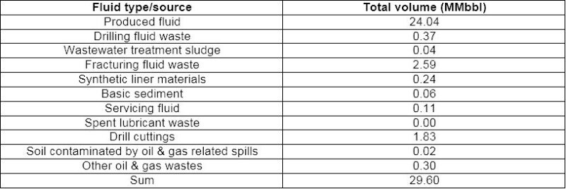
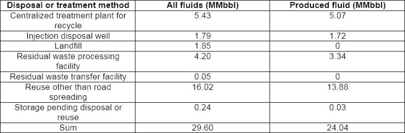
Tables 1 and 2 present summaries of the produced fluid types, volumes, and the treatment and disposal activity from mid-2015 to mid-2016. The total volume of produced water in this period was about 29.6 million bbl, of which approximately 24 million bbl were produced formation water. Most of the produced water—about 13.9 million bbl—was reused for fracturing at the same wellsite or at another wellsite. The remaining 10.1 million bbl were transferred to treatment facilities or disposal wells.
Ettehadtavakkol said there were several challenges to integrating this data into an analytic workflow. Water production in Pennsylvania is poorly reported in the public domain. Water production, recycling, and disposal data for West Virginia wells, which comprise a significant portion of the Marcellus dataset, are not publicly available. Fluid production, use, treatment, and disposal data are not available for all leases, though Ettehadtavakkol and Jamali wrote that records improved after mid-2015, implying that the usable portion of data for a reliable analysis is limited to a year-long interval from mid-2015 to mid-2016.
“Oil and gas data is sporadic and highly diversified in nature,” Ettehadtavakkol said. “There is a lot of missing data and a lot of reporting issues. We have two solutions. We can either give up on that or try to mitigate by utilizing what we have. We can use the more sophisticated databases that are available from states and companies. Our challenge is: When we acquire data, how do we handle it?”
Solving the Data Challenges
Ettehadtavakkol said that estimating produced water production was not possible without West Virginia water production data, so he and Jamali establishrd a workflow that could mitigate datasets with frequent missing or erroneous data. They started by selecting four counties in Pennsylvania near the West Virginia border (Allegheny, Fayette, Greene, and Washington) as their study area. Then they correlated annual water production and gas production data spatially and temporally. Ettehadtavakkol said that the analysis of this data indicated the significant influence of technology development on production. After dividing well production data even further (pre-2011 completed wells vs. post-2011 completed wells), he said there was a positive correlation between gas and water flow rates.
“It gives us some confidence in the use of gas flow rates to determine water flow rates. That’s a starting point. If we have more information on the completion and the wellheads, we can add that. We consider this as an extension of our work,” Ettehadtavakkol said.
Predictive models for existing wells were handled with decline curves from sample wells in each county, and water production rates were correspondingly projected with the correlation of recent wells. Ettehadtavakkol and Jamali then simulated projection of gas and water production from new wells with a five-step procedure. The first step was to average the number of wells drilled each month. Second, they assigned a gas production profile to each new well drilled in accordance to the P50 gas production profile for that county. Third, they estimated the yearly gas production of each new well. Fourth, they used a yearly water/gas correlation for each county to estimate the produced water using the estimated gas production. The last step was to add produced water from all wells to determine the county-level water production.
The annual water production predictions determined that produced water from new wells in the four counties should peak in 2020 and decline afterwards. However, the predictions only extended to a 5-year period because the extent of drilling activities will be affected by the oil and gas prices and the government policies and regulations, which will make them more likely to deviate from the logistic model.
Facility Optimization Algorithm
In 2016, Ettehadtavakkol and Chad Kronkosky published a paper that examined the application of data-driven modeling and data-driven predictive analytic approaches in the analysis of saltwater disposal in Andrews County, Texas.
To help identify optimal saltwater disposal (SWD) facility site locations in the area, they developed a random search optimization algorithm that combined classic supply/demand optimization and modern heuristic optimization methods for gridded networks. The algorithm allowed for saltwater disposal transportation patterns to be accurately identified and qualified, and it provided optimization of commercial SWD facility site locations based on historical production data.
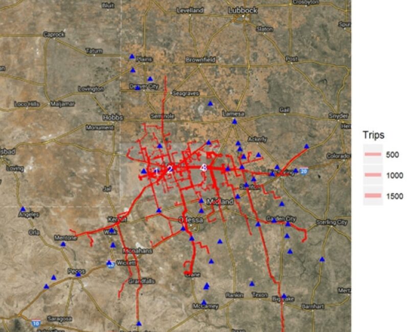
Fig. 1 shows the aggregation of fluid migration patterns and trip counts for Andrews County. Ettehadtavakkol and Kronkosky noted the distance between production locations to SWD facilities (noted as blue triangles in the figure), as well as the numerous nearby SWD disposal facility locations that various produced water transports pass on their way to their eventual disposal location. They wrote that, given this information, significant improvements could be made concerning produced water disposal hauling distances.
Ettehadtavakkol and Kronkosky used the algorithm to minimize total produced water hauling distances by optimally locating SWD facilities. They created a gridded network of site locations, randomly selected a grid cell with a positive net produced water value (grid cells where the amount of produced water was greater than the amount of injected water), and collected the nearest grid cells with positive net produced water values until their SWD facility volume constraints were met. This provided a collection of grid cells for which they could determine the optimal SWD facility site location by minimizing either the total hauling distance or total hauling duration. They wrote that using this algorithm could result in a 20% to 30% reduction in hauling distance and duration.
The algorithm did not account for produced water gathering pipelines that would ease the hauling of produced water in certain instances, though the authors noted that it could be extended to account for this case by incorporating a minimum distance threshold. They also did not account for produced water currently being disposed of at existing SWD facilities within the project extents, and that adaptations of the algorithm should account for this situation.
At URTeC, Ettehadtavakkol said that implementation of this method may result in a significant reduction in the transportation of produced water, because it will optimize recycle facility locations across the Marcellus and alter the current disposal and recycling cost structures. However, he also said implementation should be deferred due to the limited availability of public data.